Visualization walkthrough
Activate the environment
Either use docker
cd env && python launch_docker.py (--use_cuda optional)
Or activate your conda environment
source activate <conda_env_name>
Exploring the dataset
Using command line: .. code:
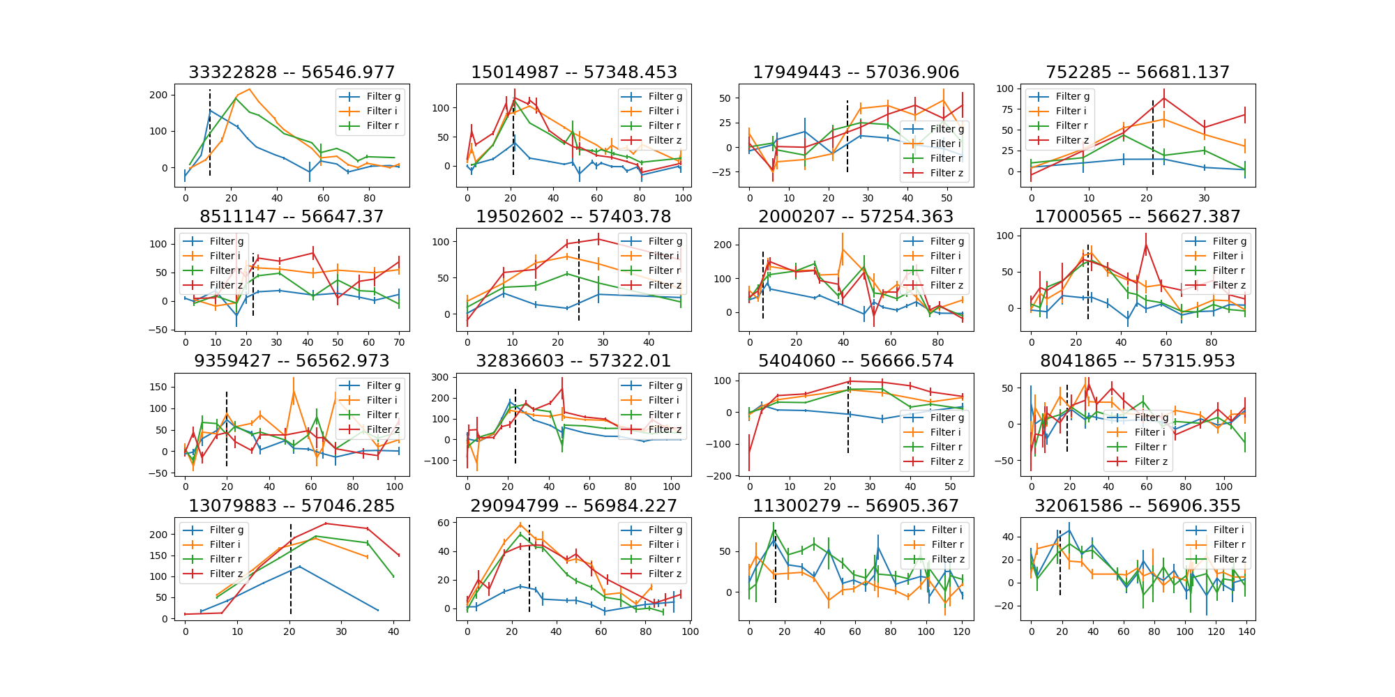
snn make_data --raw_dir tests/raw --dump_dir tests/dump --debug --explore_lightcurves
Outputs: .png files in the tests/dump/explore folder.
You should obtain something that looks like this:
Predictions as a function of time
Assuming you have a trained model stored under tests/dump/models/vanilla_S_0_CLF_2_R_None_saltfit_DF_1.0_N_global_lstm_32x2_0.05_128_True_mean
and that you have already created the database as above:
snn show --plot_lcs --dump_dir tests/dump --model_files tests/dump/models/vanilla_S_0_CLF_2_R_None_saltfit_DF_1.0_N_global_lstm_32x2_0.05_128_True_mean/vanilla_S_0_CLF_2_R_None_saltfit_DF_1.0_N_global_lstm_32x2_0.05_128_True_mean.pt
Outputs: a figure folder under tests/dump/lightcurves/vanilla_S_0_CLF_2_R_None_saltfit_DF_1.0_N_global_lstm_32x2_0.05_128_True_mean.
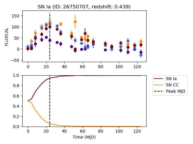
This folder contains the plot of several random lightcurves and the predictions made by the neural network referred to by the model_files argument.
If you want to plot a selection of lightcurves you can add --plot_file <filename.csv> which contains a column SNID with the ids requested to be plotted.
Below is a sample plot:
Predictions + uncertainty for bayesian models
Assuming you have a variational RNN model stored under tests/dump/models/variational_S_0_CLF_2_R_None_saltfit_DF_1.0_N_global_lstm_32x2_0.05_128_True_mean_WD_1e-07
and that you have already created the database as above:
snn show --plot_lcs --dump_dir tests/dump --model_files tests/dump/models/variational_S_0_CLF_2_R_None_saltfit_DF_1.0_N_global_lstm_32x2_0.05_128_True_mean_WD_1e-07/variational_S_0_CLF_2_R_None_saltfit_DF_1.0_N_global_lstm_32x2_0.05_128_True_mean_WD_1e-07.pt
Outputs: a figure folder under tests/dump/lightcurves/variational_S_0_CLF_2_R_None_saltfit_DF_1.0_N_global_lstm_32x2_0.05_128_True_mean_WD_1e-07.
This folder contains the plot of several lightcurves and the predictions made by the neural network referred to by the model_files argument.
Several predictions are sampled at each timestep and the prediction contours at 68% and 94% are shown.
Below is a sample plot:
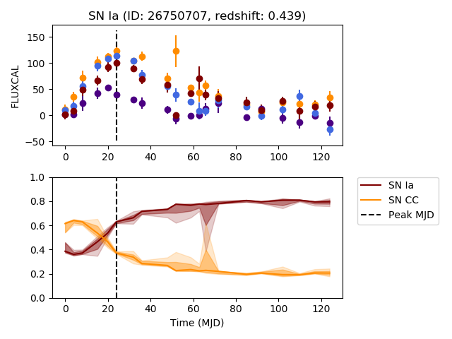
Beware: only MC Dropout (variational) and Bayes by Backprop (bayesian) models have this feature.
Predictions from multiple models
To compare the predictions from multiple models, simply call the above, while providing multiple model_files
snn show --plot_lcs --dump_dir tests/dump --model_files tests/dump/models/variational_S_0_CLF_2_R_None_saltfit_DF_1.0_N_global_lstm_32x2_0.05_128_True_mean_WD_1e-07/variational_S_0_CLF_2_R_None_saltfit_DF_1.0_N_global_lstm_32x2_0.05_128_True_mean_WD_1e-07.pt tests/dump/models/vanilla_S_0_CLF_2_R_None_saltfit_DF_1.0_N_global_lstm_32x2_0.05_128_True_mean/vanilla_S_0_CLF_2_R_None_saltfit_DF_1.0_N_global_lstm_32x2_0.05_128_True_mean.pt
Outputs: a figure folder under tests/dump/figures/multi_model_early_prediction.
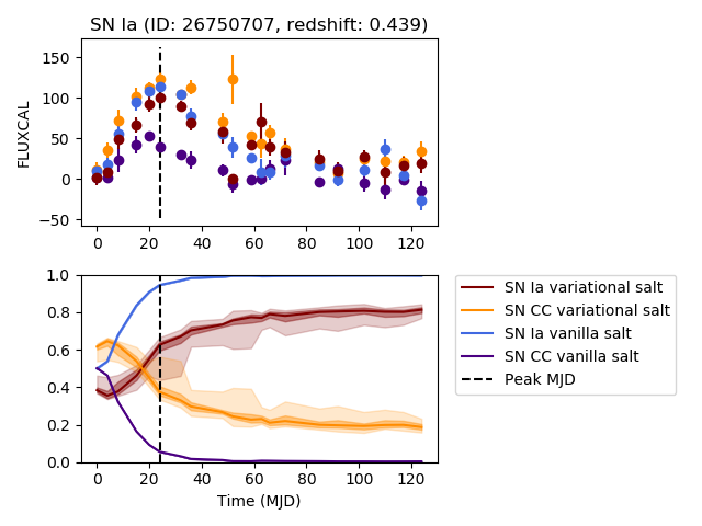
This folder contains the plot of several lightcurves and the predictions made by the neural networks referred to by the model_files argument.
Below is a sample plot:
Calibration plots for given predictions
In Calibration, we have shown how to get calibration plot while validating an RNN model or models. We can also get calibration plot by providing prediction files directly.
A prediction file looks like this: PRED_{model_name}.pickle. For instance: PRED_DES_vanilla_S_0_CLF_2_R_None_saltfit_DF_1.0_N_global_lstm_32x2_0.05_128_True_mean.pickle
Multiple prediction files can be specified, the results will be charted on the same graph.
Assuming database has been created, and prediction files have been generated.
snn show --dump_dir tests/dump --calibration --prediction_files tests/dump/models/variational_S_0_CLF_2_R_none_photometry_DF_1.0_N_global_lstm_32x2_0.05_128_True_mean_WD_1e-07/PRED_variational_S_0_CLF_2_R_none_photometry_DF_1.0_N_global_lstm_32x2_0.05_128_True_mean_WD_1e-07.pickle tests/dump/vanilla_S_0_CLF_2_R_none_photometry_DF_1.0_N_global_lstm_32x2_0.05_128_True_mean/PRED_vanilla_S_0_CLF_2_R_none_photometry_DF_1.0_N_global_lstm_32x2_0.05_128_True_mean.pickle
Science plots
The plots of the paper can be reproduced by running in the paper branch:
python run_paper.py